Chapter 14 Generative DAGs As Business and Mathematical Narratives
Up to this point, we specified a prior joint distribution using information from both a graphical model and a statistical model. In this chapter, we combine the two model types, graphical models and statistical models, into one visualization called the generative DAG. Recall that DAG is an acronym for directed acyclic graph. This concept was introduced in the Graphical Models chapter. The advantage of this is that the generative DAG unites real-world measurements (e.g. getting a credit card) with their math/computation world counterparts (e.g.
14.1 Generative DAGs
*** A statistical model is a mathematically expressed recipe for creating a joint distribution of related random variables. Each variable is defined either using a probability distribution or a function of the other variables. Statistical model and generative DAG will be used interchangeably. The term statistical model is just the mathematically expressed recipe. Generative DAG is the graphically expressed recipe with an embedded statistical model. Note: Most terms used in this book are commonplace in other texts. However, the definition of generative DAGs is unique to this text. Most other textbooks will refer to these as Bayesian networks or DAGs, but the statistical model is often presented separately or via less intuitive factor graphs. In later chapters, the causact package in R will be used to quickly create these generative DAGs and to automate the accompanying computer code. As we will see, this use of generative DAGs accelerates the BAW more than any other representation.
To build a generative DAG, we combine a graphical model with a statistical model
The creation of a generative DAG mimics the creation of graphical models with accompanying statistical models. Both the structure of the DAG and the definition of the random variables should reflect what a domain expert knows, or wants to assume, about the business narrative being investigated.
Figure 14.1: The Chili’s model as a generative DAG.
Recall the Chili’s example from the previous chapter. Figure 14.1 shows a generative DAG for this model. Some elements of this DAG are easily digested as we have seen them before. For example, the Sales Increase (
Other elements of the DAG are new. Notice, theta is now spelled out phonetically as opposed to using the actual Greek letter math symbol of theta here because computer code and computer-generated DAG visuals lack easy support for the Greek alphabet. Additionally, and more importantly, we switch to using lowercase notation for both x and theta as we want to highlight that basic ovals in generative DAG models represent a single realization of the random variable. Our mental models for generative DAGs should think of the basic oval representing a single realization. Later chapters will introduce the representation of more than one realization.
14.2 Building Generative Models
As we build these models, it is often easiest to build and read them from bottom to top; start by converting your target measurement, in this case whether a store increases sales, to a brief real-world description (e.g. Sales Increase). This description is the top-line of the oval. For rigor, a more formal definition should be stored outside of the generative DAG in a simple text document that can be referenced by others.
14.2.1 Structuring The Mathematical Line
Every node will also have a mathematical line (e.g. x ~ Bernoulli(theta)). The mathematical line will always follow a three-part structure of 1) Left-hand side, 2) Relationship Type, and 3) Right-hand side:
Each line of a statistical model follows one of two forms:
- Left-hand side (LHS): a mathematical label for a realization of the node (e.g.
- Relationship Type: There are two types of relationships that can be specified:
- a probabilistic relationship, denoted by the
- a deterministic relationship denoted by an
- Right-hand side (RHS): either a known probability distribution governing the node’s probabilistic outcome (e.g.
14.3 Defining Missing Parent Nodes
To model subsequent nodes, consider any parameters or variables on the right-hand side of the mathematical lines that remain undefined; all of these undefined parameters must be defined on the LHS of a parent node. Hence, for
To learn more about the uniform distribution or any common probability distribution, consult Wikipedia; e.g. https://en.wikipedia.org/wiki/Continuous_uniform_distribution. The Wikipedia entry for every distribution has a nice graph for the probability density function (PDF) and also explicit formula, when available, for the PDF,CDF,mean,etc. on the right side. It is a great resource that even mathematicians refer to regularly.
Now to have a complete statistical model, we need a recipe for how all the random variables of interest can be generated. Previously, when doing Bayes rule calculations by hand, we considered a recipe for
Figure 14.2: A complete generative DAG for the Chili’s model.
Figure 14.2 provides a complete mathematical line for
14.4 Using The Generative Recipe
Notice that the generative DAG is a recipe for simulating or generating a single sample from the joint distribution - read it from top-to-bottom: 1) first, simulate a random sample value of
For illustrating the generative aspect of a generative DAG, we can use simple R functions to get a joint realization of the two variables. We model runif and rbern (i.e. rfoo for the uniform distribution and Bernoulli distribution, respectively). Hence, a random sample from the joint distribution for realizations
library(causact) # used for rbern function
set.seed(1234)

# generate random theta: n is # of samples we want
theta = runif(n=1,min=0,max=1)
theta # print value
## [1] 0.1137034## [1] 0For the particular model above, the recipe picked a random
## [1] 0 0 0 0 0 0 0 0 0 0 0 1Generative models are abstractions of a business problem. We will use these abstractions and Bayesian inference via computer to combine prior information in the form of a generative DAG and observed data. The combination will yield us a posterior distribution; a joint distribution over our RV’s of interest that we can use to answer questions and generate insight. For most generative DAGs, Bayes rule is not analytically tractable (i.e. it can’t be reduced to simple math), and we need to define a computational model. This is done in greta and is demonstrated in the next two chapters.
14.5 Representing Observed Data With Fill And A Plate
Figure 14.2 provides a generative recipe for simulating a real-world observation. As in the Bayesian Inference chapter, we can then use data to inform us about which of the generatable recipes seem more consistent with the data. For example, we know that the success of three stores in a row would be very inconsistent with a recipe based on the pessimist model. Thus, reallocating plausibility in light of this type of data becomes a milestone during our data analysis.
For the Chili’s model, the reallocation of probability in light of data from three stores will be done in such a way as to give more plausibility to
Figure 14.3: A complete generative DAG for the Chili’s model.
First, the
In Figure 14.3, there are some additional elements shown in the generative DAG. Observed data - in contrast to latent parameters or unobserved data - gets represented by using fill shading of the ovals (e.g. the darker fill of
The
Text in the lower right-hand corner of the plate indicates how variables inside the plate are repeated and indexed. In this case, there will be one realization of x[i] is the x and therefore, x[2] would the x. The [3] in the lower-right hand corner represents the number of repetitions of the RV, in this case there are 3 observations of stores: x[1], x[2], and x[3].
Since the
14.6 Digging Deeper
More rigorous mathematical notation and definitions can be found in the lucid recommendations of Michael Betancourt. See his work Towards a Principled Bayesian Workflow (Rstan) for a more in-depth treatment of how generative models and prior distributions are only models of real-world processes. https://betanalpha.github.io/assets/case_studies/principled_bayesian_workflow.html. Additionally, Betancourt’s Generative Modelling (https://betanalpha.github.io/assets/case_studies/generative_modeling.html) is excellent in explaining how models with narrative interpretations tell a set of stories on how data are generated. For us, we will combine our generative DAGs with observed data to refine our beliefs about which stories (i.e. which parameters) seem more plausible than others. Additionally, sometimes
14.7 Exercises
Figure 14.4: A generative recipe for simulating the time a car spends at a car wash.
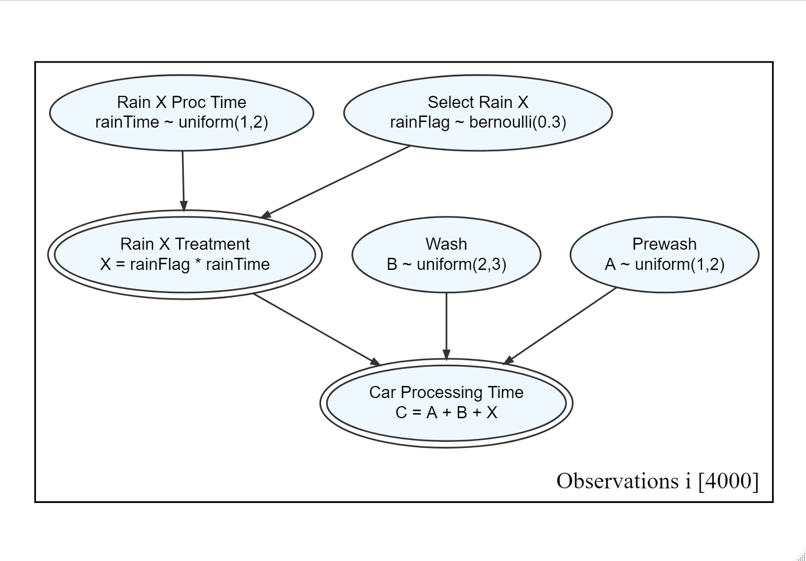
Exercise 14.1 Write R code using runif() and causact::rbern() to follow the generative recipe of Figure 14.4 that will generate 4,000 draws (i.e. realizations) of the “C” random variable representing the processing time of an individual car.
For example, this code will generate 4,000 draws of rainTime:
After simulating 4,000 draws for the entire car wash process, what percentage of those draws have a car processing time GREATER than 6 minutes? Report your percentage as a decimal with three significant digits (e.g. enter 0.342 for 34.2%). Since there is some randomness in your result, a range of answers are acceptable.